Understanding Dimension Importance Estimation (DIME) for Dense Information Retrieval through Code and Experimentation
Introduction
Dense embedding-based retrieval is being widely adapted in recent days. Unlike traditional sparse methods like BM25, which are based on lexical matching, dense embeddings capture semantic relationships and represent data in fixed-sized vectors ranging from a few hundreds to a few thousands. Each coordinate/dimension in the learned representation corresponds to some latent feature of the input data. For example, when text data is encoded into dense embeddings, it could represent various linguistic features, semantic meaning, conceptual features, etc. These are represented as floating numbers in vectors and are almost impossible for humans to interpret what the numbers actually encode.
This is one of the main reasons why dense embeddings tend to be more powerful than traditional methods, but in recent few years, people started noticing the noise these dense embeddings introduce along with the features. Let’s say when a query is represented with a dense embedding, only some part of the embedding could encode meaningful features, and the rest can be noise. When the same embedding is used to retrieve documents, the retrieval can be poor because of the noise. Hence, it is essential to keep only dimensions which encode meaningful features and exclude noise during retrieval.
But as I mentioned earlier, these embeddings are learned representations (mostly from deep learning models) which encode latent features; identifying the meaningful dimensions is not straightforward.
A paper released in 2024 called “Dimension Importance Estimation for Dense Information Retrieval” proposes various approaches to prune irrelevant dimensions. Recently, Pinecone did some deeper analysis on these approaches and released another paper with code. In this article, I’ll be going through some of the key details from these.
DIME Framework
A simple goal here is to identify all irrelevant features (noise) from the dense embedding and zero them out to create another dense embedding which contains only the relevant features.
In a typical workflow, documents are embedded and stored. A query is embedded and queried on documents to retrieve relevant documents.
When the query is converted to an embedding, the DIME framework takes the query embedding, applies one of the below approaches, and transforms the query embedding by zeroing out all irrelevant dimensions.
In short, DIME acts on query embedding on the fly, thus requiring no retraining or reindexing. Once the query embedding is transformed, it can be either used for reranking or refetching.
1
Q = [q1, q2, q3, q4, q5, q6] -> [q1, 0, q3, q4, 0, 0]
Appraoches
- Magnitude DIME
- PRF DIME
- LLM DIME
- Active Feedback DIME
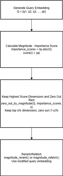
Magnitude DIME
It is one of the simplest methods; here, the magnitude of the dimension is used to determine the importance of the dimension. The assumption is: the larger the magnitude, the more important the dimension is; lesser magnitude dimensions are noise or less relevant.
1
q(i) = ∣qi∣ for all i∈[1,N] where N is the total number of dimensions in Q.
This method relies solely on the query embedding itself to determine the importance of the dimension; the rest of all methods require another reference embedding which helps in deciding the importance of the dimension.
Click to expand: Magnitude based DIME implementation
1
2
3
4
5
6
7
8
9
10
11
12
13
14
15
16
17
18
19
20
21
22
23
24
25
26
27
28
29
30
31
32
33
34
35
36
37
38
39
40
41
42
43
44
45
46
47
48
49
50
51
52
53
54
55
56
57
58
59
60
61
62
63
64
65
66
67
68
69
70
71
72
73
74
75
76
77
78
79
80
81
82
83
84
85
86
87
88
89
class MagnitudeBasedDIME:
    ...
    def magnitude_rerank(self, query, initial_top_k=1000, final_top_k=10, zero_out_ratio=0.2):
        # Compute dimension importance using magnitude
        print(f"Computing dimension importance using magnitude...")
        importance_scores = np.abs(original_query_embedding)

        # Zero out least important dimensions based on magnitude
        print(f"Zeroing out {zero_out_ratio*100}% least important dimensions...")
        alpha = 1 - zero_out_ratio
        modified_query_embedding = self._zero_out_by_magnitude(original_query_embedding, importance_scores, alpha)

        # Re-score all initial results with modified query
        print(f"Re-scoring with modified query...")
        reranked_results = []
        for result in initial_results:
            new_score = float(np.dot(modified_query_embedding, result['embedding']))
            reranked_results.append({
                'rank': result['rank'],
                'index': result['index'],
                'product_id': result['product_id'],
                'title': result['title'],
                'original_score': result['score'],
                'new_score': new_score
            })

        # Sort by new scores and take top-k
        reranked_results.sort(key=lambda x: -x['new_score'])
        final_results = reranked_results[:final_top_k]
        ...

    def magnitude_refetch(self, query, final_top_k=10, zero_out_ratio=0.2):
        # Compute dimension importance using magnitude
        print(f"Computing dimension importance using magnitude...")
        importance_scores = np.abs(original_query_embedding)

        # Zero out least important dimensions based on magnitude
        print(f"Zeroing out {zero_out_ratio*100}% least important dimensions...")
        alpha = 1 - zero_out_ratio
        modified_query_embedding = self._zero_out_by_magnitude(original_query_embedding, importance_scores, alpha)

        # Perform new retrieval with modified query
        print(f"Performing new retrieval with modified query...")
        refetch_scores = np.dot(self.embeddings, modified_query_embedding)
        top_indices = np.argsort(refetch_scores)[::-1][:final_top_k]

        refetched_results = []
        for i, idx in enumerate(top_indices):
            refetched_results.append({
                'rank': i + 1,
                'index': idx,
                'product_id': self.df.iloc[idx]['product_id'],
                'title': self.df.iloc[idx]['title'],
                'score': refetch_scores[idx]
            })
        ...

    def _zero_out_by_magnitude(self, query_vector, importance_scores, alpha=0.8):
        """
        Zero out the lowest (1-alpha) fraction of dimensions based on magnitude importance

        Args:
            query_vector: Original query vector
            importance_scores: Magnitude-based importance scores (|qi|)
            alpha: Fraction of dimensions to keep (0.8 means keep 80%)

        Returns:
            Modified query vector with least important dimensions zeroed out
        """
        dim = len(importance_scores)
        keep_count = int(alpha * dim)

        if keep_count >= dim:
            return query_vector.copy()

        # Get indices of most important dimensions (highest magnitude)
        sorted_indices = np.argsort(importance_scores)
        keep_indices = set(sorted_indices[-keep_count:])

        # Zero out least important dimensions
        modified_query_vector = query_vector.copy()
        for i in range(dim):
            if i not in keep_indices:
                modified_query_vector[i] = 0.0

        return modified_query_vector
# Initialize Magnitude-based DIME
magnitude_dime = MagnitudeBasedDIME(model, product_embeddings, df)
print("Magnitude-based DIME initialized successfully!")
Here, zero_out_ratio is a hyperparameter which tells how many dimensions to prune. The same hyperparameter is used across all methods.
Note: It is important to keep in mind that none of the approaches exactly pinpoint whether a dimension is important or not; it is all relative, so it is us who decide what fraction of dimensions to prune, depending on how important we decide it is and how we decide that is using these 4 approaches.
Before we move to next approaches, I want to recall one of the points I mentioned earlier: to determine the importance of the dimension, all approaches except Magnitude DIME rely on a reference embedding. All 3 upcoming approaches differ in the way how they construct that reference embedding, and rest all concepts remain more or less same.
Why Reference Embedding Needed?
In order to determine the importance of a dimension, we need some sort of scoring mechanism which assigns scores to each dimension, and then we can prune a percentage of dimensions with less score. In the previous approach, we directly considered magnitude as the score, but in rest of the approaches, we rely on some reference embedding and then calculate the score of the dimension by performing element-wise multiplication — [qi⋅ri]. Hence, we need to make sure that the reference embedding can’t be just some random embedding; instead, it should be something relevant to the query embedding.
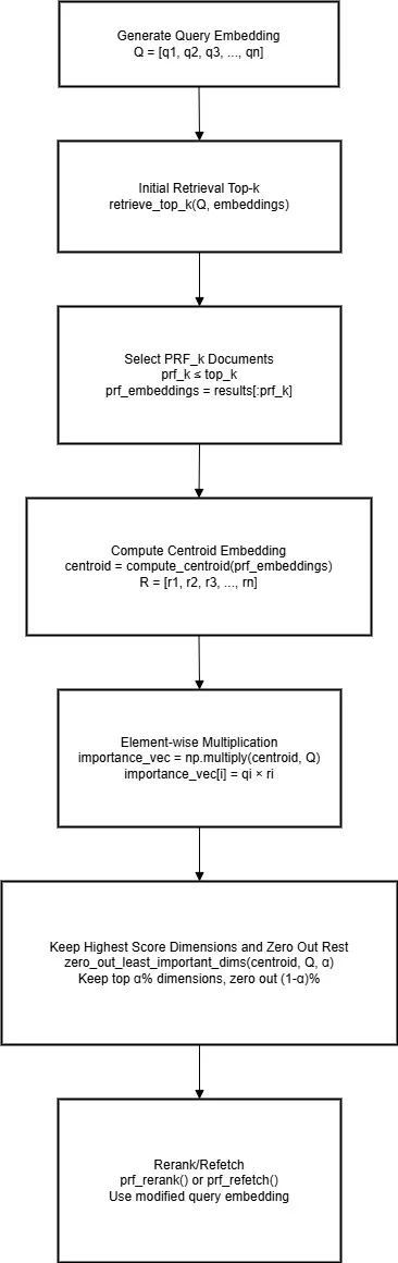
PRF (Pseudo-Relevance Feedback) DIME
This approach is based on the assumption that the initial documents of the top-k retrieved documents are most likely to be relevant to the query. Here, we take prf_k (prf ≤ top-k), compute a centroid embedding from these embeddings, and consider this centroid embedding as the reference embedding, which is then used to calculate the dimension score by performing element-wise multiplication.
Click to expand: PRF based DIME implementation
1
2
3
4
5
6
7
8
9
10
11
12
13
14
15
16
17
18
19
20
21
22
23
24
25
26
27
28
29
30
31
32
def zero_out_least_important_dims(centroid, query_vector, alpha=0.8):
    """
    Zero out the lowest (1-alpha) fraction of dimensions in query_vector
    based on element-wise product between centroid and query_vector

    Args:
        centroid: Centroid vector for dimension importance
        query_vector: Original query vector
        alpha: Fraction of dimensions to keep (0.8 means keep 80%)

    Returns:
        Modified query vector with least important dimensions zeroed out
    """
    # Element-wise product to determine dimension importance
    importance_vec = np.multiply(centroid, query_vector)
    dim = len(importance_vec)
    keep_count = int(alpha * dim)

    if keep_count >= dim:
        return query_vector.copy()

    # Get indices of most important dimensions
    sorted_indices = np.argsort(importance_vec)
    keep_indices = set(sorted_indices[-keep_count:])

    # Zero out least important dimensions
    modified_query_vector = query_vector.copy()
    for i in range(dim):
        if i not in keep_indices:
            modified_query_vector[i] = 0.0

    return modified_query_vector
1
2
3
4
5
6
7
8
9
10
11
12
13
14
15
16
17
18
19
20
21
22
23
24
25
26
27
28
29
30
31
32
33
34
35
36
37
38
39
40
41
42
43
44
45
46
47
48
49
50
51
52
53
54
55
56
57
58
59
60
61
62
63
64
65
66
67
68
69
70
71
72
73
class PRFBasedDIME:
    ...

    def prf_rerank(self, query, initial_top_k=1000, prf_k=10, final_top_k=10,
                   zero_out_ratio=0.2, weighted=False, attention_type="linear", temperature=1.0):
        # Compute centroid from top-k PRF documents
        print(f"Computing centroid from top-{prf_k} PRF documents...")
        prf_embeddings = np.array([r['embedding'] for r in initial_results[:prf_k]])
        prf_scores = np.array([r['score'] for r in initial_results[:prf_k]])

        centroid = compute_centroid(prf_embeddings, prf_scores, k=None,
                                  weighted=weighted, attention_type=attention_type,
                                  temperature=temperature)

        # Zero out least important dimensions
        print(f"Zeroing out {zero_out_ratio*100}% least important dimensions...")
        alpha = 1 - zero_out_ratio
        modified_query_embedding = zero_out_least_important_dims(centroid, original_query_embedding, alpha)

        # Re-score all initial results with modified query
        print(f"Re-scoring with modified query...")
        reranked_results = []
        for result in initial_results:
            new_score = float(np.dot(modified_query_embedding, result['embedding']))
            reranked_results.append({
                'rank': result['rank'],
                'index': result['index'],
                'product_id': result['product_id'],
                'title': result['title'],
                'original_score': result['score'],
                'new_score': new_score
            })

        # Sort by new scores and take top-k
        reranked_results.sort(key=lambda x: -x['new_score'])
        final_results = reranked_results[:final_top_k]

        ...

    def prf_refetch(self, query, initial_top_k=1000, prf_k=10, final_top_k=10,
                    zero_out_ratio=0.2, weighted=False, attention_type="linear", temperature=1.0):
        # Compute centroid from top-k PRF documents
        print(f"Computing centroid from top-{prf_k} PRF documents...")
        prf_embeddings = np.array([r['embedding'] for r in initial_results[:prf_k]])
        prf_scores = np.array([r['score'] for r in initial_results[:prf_k]])

        centroid = compute_centroid(prf_embeddings, prf_scores, k=None,
                                  weighted=weighted, attention_type=attention_type,
                                  temperature=temperature)

        # Zero out least important dimensions
        print(f"Zeroing out {zero_out_ratio*100}% least important dimensions...")
        alpha = 1 - zero_out_ratio
        modified_query_embedding = zero_out_least_important_dims(centroid, original_query_embedding, alpha)

        # Perform new retrieval with modified query
        print(f"Performing new retrieval with modified query...")
        refetch_scores = np.dot(self.embeddings, modified_query_embedding)
        top_indices = np.argsort(refetch_scores)[::-1][:final_top_k]

        refetched_results = []
        for i, idx in enumerate(top_indices):
            refetched_results.append({
                'rank': i + 1,
                'index': idx,
                'product_id': self.df.iloc[idx]['product_id'],
                'title': self.df.iloc[idx]['title'],
                'score': refetch_scores[idx]
            })
        ...
# Initialize PRF-based DIME
prf_dime = PRFBasedDIME(model, product_embeddings, df)
print("PRF-based DIME initialized successfully!")
Here, Pinecone proposed an enhancement in calculating the centroid of the prf_k document embeddings. In the original paper, centroid calculation was just an arithmetic mean, but considering that in top-k documents not all documents are equally relevant to the query (the first document is highly relevant than the third one, for example), providing some weight for each document embedding can improve the reference embedding quality furthermore. To calculate this weight, Pinecone proposed simple linear weighting and softmax-based weighting methods.
More about the implementation of the weighting logic can be found here.
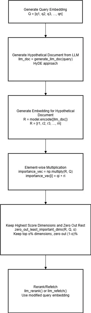
LLM DIME
If you have worked on RAG, you would have probably heard of a technique called Hypothetical Document Embeddings (HyDE). In a typical scenario, a query is converted to an embedding and then used to retrieve a document. This could lead to asymmetric search where the query can be small and documents can be large. To tackle this, HyDE can be helpful. Here, an LLM is instructed to generate a Hypothetical Document for the query, which is then encoded and used for retrieval.
In this approach, the encoded Hypothetical Document can be used as a reference embedding to determine dimension importance. This completely makes sense because the main criteria for a reference embedding is that it should be relevant to the query embedding. In the PRF DIME approach, we used top relevant documents to calculate that, but here we use an LLM to create that document.
Click to expand: LLM based DIME implementation
1
2
3
4
5
6
7
8
9
10
11
12
13
14
15
16
17
18
19
20
21
22
23
24
25
26
27
28
29
30
31
32
33
34
35
36
37
38
39
40
41
42
43
44
45
46
47
48
49
50
51
52
53
54
55
56
57
58
59
60
61
62
63
64
65
66
67
68
69
70
71
72
73
74
75
76
77
78
79
80
81
82
83
84
class LLMBasedDIME:
    ...

    def generate_llm_doc(self, query):
        """
        Generate LLM-style document for the query
        Since we don't have actual LLM, we'll simulate by creating expanded query
        """
        # Simple expansion - in real implementation, this would use an LLM
        expanded_queries = {
            "black dress shirt": "elegant black dress shirt formal business professional men's clothing cotton long sleeve button up office wear",
            "blue jeans": "blue denim jeans casual wear pants trousers men women comfortable cotton everyday fashion",
            "white sneakers": "white athletic sneakers shoes casual sports footwear comfortable rubber sole walking running",
            "red dress": "red dress women's formal elegant party evening wear special occasion outfit stylish",
            "brown leather boots": "brown leather boots shoes footwear men's outdoor durable sturdy walking hiking",
            "casual t-shirt": "casual t-shirt comfortable cotton everyday wear men women basic wardrobe essential",
            "winter coat": "winter coat warm jacket outerwear cold weather protection insulated heavy duty",
            "summer dress": "summer dress light breathable women's warm weather casual comfortable seasonal clothing"
        }


        return expanded_queries[query]

    def llm_rerank(self, query, initial_top_k=1000, final_top_k=10, zero_out_ratio=0.2):
        # Generate LLM document and embed it
        print(f"Generating and embedding LLM document...")
        llm_doc = self.generate_llm_doc(query)
        print(f"Generated LLM doc: {llm_doc}")
        llm_embedding = self.model.encode([llm_doc], normalize_embeddings=True)[0]

        # Zero out least important dimensions using LLM embedding
        print(f"Zeroing out {zero_out_ratio*100}% least important dimensions...")
        alpha = 1 - zero_out_ratio
        modified_query_embedding = zero_out_least_important_dims(llm_embedding, original_query_embedding, alpha)

        # Re-score all initial results with modified query
        print(f"Re-scoring with modified query...")
        reranked_results = []
        for result in initial_results:
            new_score = float(np.dot(modified_query_embedding, result['embedding']))
            reranked_results.append({
                'rank': result['rank'],
                'index': result['index'],
                'product_id': result['product_id'],
                'title': result['title'],
                'original_score': result['score'],
                'new_score': new_score
            })

        # Sort by new scores and take top-k
        reranked_results.sort(key=lambda x: -x['new_score'])
        final_results = reranked_results[:final_top_k]
        ...

    def llm_refetch(self, query, final_top_k=10, zero_out_ratio=0.2):
        # Generate LLM document and embed it
        print(f"Generating and embedding LLM document...")
        llm_doc = self.generate_llm_doc(query)
        print(f"Generated LLM doc: {llm_doc}")
        llm_embedding = self.model.encode([llm_doc], normalize_embeddings=True)[0]

        # Zero out least important dimensions using LLM embedding
        print(f"Zeroing out {zero_out_ratio*100}% least important dimensions...")
        alpha = 1 - zero_out_ratio
        modified_query_embedding = zero_out_least_important_dims(llm_embedding, original_query_embedding, alpha)

        # Perform new retrieval with modified query
        print(f"Performing new retrieval with modified query...")
        refetch_scores = np.dot(self.embeddings, modified_query_embedding)
        top_indices = np.argsort(refetch_scores)[::-1][:final_top_k]

        refetched_results = []
        for i, idx in enumerate(top_indices):
            refetched_results.append({
                'rank': i + 1,
                'index': idx,
                'product_id': self.df.iloc[idx]['product_id'],
                'title': self.df.iloc[idx]['title'],
                'score': refetch_scores[idx]
            })
        ...
# Initialize LLM-based DIME
llm_dime = LLMBasedDIME(model, product_embeddings, df)
print("LLM-based DIME initialized successfully!")
Active-Feedback DIME
This method is very much similar to LLM DIME, but here instead of using an LLM to generate a relevant document, a human-assessed document is considered as the reference document. This might be useful in scenarios where a user asks a question and the search engine returns results. If the user then clicks on one of them, the document user clicked can be considered as the relevant document, and then the results can be refined.
Results Comparison
We have covered all four approaches, and I’ve conducted small experiments on my end on some sample data to quickly check the results.
Click to expand: Full results comparison
1
2
3
4
5
6
7
8
9
10
11
12
13
14
15
16
17
18
19
20
21
22
23
24
25
26
27
28
29
30
31
32
33
34
35
36
37
38
39
40
41
42
43
44
45
46
47
48
49
50
51
52
53
54
55
56
57
58
59
60
61
62
63
64
65
66
67
68
69
70
71
72
73
74
75
76
77
78
79
80
81
82
83
84
85
86
87
88
89
90
91
92
93
94
95
96
97
98
99
100
101
102
103
104
105
106
107
108
109
110
111
112
113
114
115
116
117
118
119
120
121
122
123
124
125
126
127
128
129
130
131
132
133
134
135
136
137
138
139
140
141
142
143
144
145
146
147
148
149
150
151
152
153
154
155
156
157
158
159
160
161
162
163
164
165
166
167
168
169
170
171
172
173
174
175
176
177
178
179
180
181
182
183
184
185
186
187
188
189
190
191
192
193
194
195
196
197
198
199
200
201
202
203
204
205
206
207
208
209
210
211
212
213
214
215
216
217
218
219
220
221
222
223
224
225
226
227
228
229
230
231
232
233
234
235
236
237
238
239
240
241
242
243
244
245
246
247
248
249
250
251
252
253
254
255
256
257
258
259
260
261
262
263
264
265
266
267
268
269
270
271
272
273
274
275
276
277
278
279
280
281
282
283
284
285
286
287
288
289
290
291
292
293
294
295
296
297
298
299
300
301
302
303
304
305
306
307
308
309
310
311
312
313
314
315
316
317
318
319
320
321
322
323
324
325
326
327
328
329
330
331
332
333
334
335
336
337
338
339
340
341
342
343
344
345
346
347
348
349
350
351
352
353
354
355
356
357
358
359
360
361
362
363
364
365
366
367
368
369
370
371
372
373
374
375
376
377
378
379
380
381
382
383
384
385
386
test_queries = [    "black dress shirt",
    "blue jeans",
    "white sneakers",
    "red dress",
    "casual t-shirt",
    "winter coat",
    "summer dress",
]
================================================================================
RESULTS COMPARISON FOR: 'black dress shirt'
================================================================================
BASELINE (Original Dense Retrieval):
--------------------------------------------------
1. J.Crew Black Blouses - Score: 0.5945
2. Gap Black Blouses - Score: 0.5807
3. Hollister Black T-Shirts in Viscose - Score: 0.5762
4. American Eagle Black T-Shirts - Score: 0.5690
5. Burberry Black Casual Shirts in Viscose - Score: 0.5592
MAGNITUDE RERANK:
--------------------------------------------------
1. J.Crew Black Blouses - Score: 0.5763
2. American Eagle Black T-Shirts - Score: 0.5584
3. Hollister Black T-Shirts in Viscose - Score: 0.5565
4. Gap Black Blouses - Score: 0.5536
5. Burberry Black Casual Shirts in Viscose - Score: 0.5353
MAGNITUDE REFETCH:
--------------------------------------------------
1. J.Crew Black Blouses - Score: 0.5763
2. American Eagle Black T-Shirts - Score: 0.5584
3. Hollister Black T-Shirts in Viscose - Score: 0.5565
4. Gap Black Blouses - Score: 0.5536
5. Burberry Black Casual Shirts in Viscose - Score: 0.5353
PRF RERANK:
--------------------------------------------------
1. Hollister Black T-Shirts in Viscose - Score: 0.6360
2. J.Crew Black Blouses - Score: 0.6217
3. American Eagle Black T-Shirts - Score: 0.6179
4. Burberry Black Casual Shirts in Viscose - Score: 0.6054
5. Gap Black Blouses - Score: 0.6006
PRF REFETCH:
--------------------------------------------------
1. Hollister Black T-Shirts in Viscose - Score: 0.6360
2. J.Crew Black Blouses - Score: 0.6217
3. American Eagle Black T-Shirts - Score: 0.6179
4. Burberry Black Casual Shirts in Viscose - Score: 0.6054
5. Gap Black Blouses - Score: 0.6006
LLM RERANK:
--------------------------------------------------
1. J.Crew Black Blouses - Score: 0.5135
2. Hollister Black Swimwear - Score: 0.5121
3. Burberry Black Casual Shirts in Viscose - Score: 0.5108
4. Hollister Black T-Shirts in Viscose - Score: 0.5010
5. American Eagle Black T-Shirts - Score: 0.4955
   LLM Doc: elegant black dress shirt formal business professional men's clothing cotton long sleeve button up o...
LLM REFETCH:
--------------------------------------------------
1. J.Crew Black Blouses - Score: 0.5135
2. Hollister Black Swimwear - Score: 0.5121
3. Burberry Black Casual Shirts in Viscose - Score: 0.5108
4. Hollister Black T-Shirts in Viscose - Score: 0.5010
5. American Eagle Black T-Shirts - Score: 0.4955
   LLM Doc: elegant black dress shirt formal business professional men's clothing cotton long sleeve button up o...
================================================================================
RESULTS COMPARISON FOR: 'blue jeans'
================================================================================
BASELINE (Original Dense Retrieval):
--------------------------------------------------
1. Gap Blue Jeans in Suede - Score: 0.6695
2. Hollister Blue Jeans in Acrylic - Score: 0.6394
3. COS Blue Jeans in Wool - Score: 0.6391
4. J.Crew Blue Skirts in Denim - Score: 0.6225
5. COS Purple Jeans - Score: 0.6168
MAGNITUDE RERANK:
--------------------------------------------------
1. Gap Blue Jeans in Suede - Score: 0.6434
2. Hollister Blue Jeans in Acrylic - Score: 0.6290
3. COS Blue Jeans in Wool - Score: 0.6151
4. PrettyLittleThing Brown Jeans - Score: 0.6008
5. J.Crew Blue Skirts in Denim - Score: 0.6000
MAGNITUDE REFETCH:
--------------------------------------------------
1. Gap Blue Jeans in Suede - Score: 0.6434
2. Hollister Blue Jeans in Acrylic - Score: 0.6290
3. COS Blue Jeans in Wool - Score: 0.6151
4. PrettyLittleThing Brown Jeans - Score: 0.6008
5. J.Crew Blue Skirts in Denim - Score: 0.6000
PRF RERANK:
--------------------------------------------------
1. Gap Blue Jeans in Suede - Score: 0.6818
2. Hollister Blue Jeans in Acrylic - Score: 0.6659
3. COS Blue Jeans in Wool - Score: 0.6616
4. J.Crew Blue Skirts in Denim - Score: 0.6437
5. COS Purple Jeans - Score: 0.6362
PRF REFETCH:
--------------------------------------------------
1. Gap Blue Jeans in Suede - Score: 0.6818
2. Hollister Blue Jeans in Acrylic - Score: 0.6659
3. COS Blue Jeans in Wool - Score: 0.6616
4. J.Crew Blue Skirts in Denim - Score: 0.6437
5. COS Purple Jeans - Score: 0.6362
LLM RERANK:
--------------------------------------------------
1. Gap Blue Jeans in Suede - Score: 0.6223
2. Hollister Blue Jeans in Acrylic - Score: 0.6096
3. COS Blue Jeans in Wool - Score: 0.5948
4. COS Purple Jeans - Score: 0.5812
5. J.Crew Blue Skirts in Denim - Score: 0.5741
   LLM Doc: blue denim jeans casual wear pants trousers men women comfortable cotton everyday fashion...
LLM REFETCH:
--------------------------------------------------
1. Gap Blue Jeans in Suede - Score: 0.6223
2. Hollister Blue Jeans in Acrylic - Score: 0.6096
3. COS Blue Jeans in Wool - Score: 0.5948
4. COS Purple Jeans - Score: 0.5812
5. J.Crew Blue Skirts in Denim - Score: 0.5741
   LLM Doc: blue denim jeans casual wear pants trousers men women comfortable cotton everyday fashion...
================================================================================
RESULTS COMPARISON FOR: 'white sneakers'
================================================================================
BASELINE (Original Dense Retrieval):
--------------------------------------------------
1. Gap White Sneakers - Score: 0.7189
2. Uniqlo White Sneakers in Leather - Score: 0.7051
3. COS Gray Sneakers - Score: 0.6921
4. Uniqlo White Sneakers in Polyester - Score: 0.6899
5. COS Gray Sneakers - Score: 0.6701
MAGNITUDE RERANK:
--------------------------------------------------
1. Gap White Sneakers - Score: 0.7004
2. Uniqlo White Sneakers in Leather - Score: 0.6812
3. COS Gray Sneakers - Score: 0.6802
4. Uniqlo White Sneakers in Polyester - Score: 0.6649
5. COS Gray Sneakers - Score: 0.6586
MAGNITUDE REFETCH:
--------------------------------------------------
1. Gap White Sneakers - Score: 0.7004
2. Uniqlo White Sneakers in Leather - Score: 0.6812
3. COS Gray Sneakers - Score: 0.6802
4. Uniqlo White Sneakers in Polyester - Score: 0.6649
5. COS Gray Sneakers - Score: 0.6586
PRF RERANK:
--------------------------------------------------
1. COS Gray Sneakers - Score: 0.7142
2. Gap White Sneakers - Score: 0.7111
3. Uniqlo White Sneakers in Leather - Score: 0.7105
4. Uniqlo White Sneakers in Polyester - Score: 0.6964
5. COS Gray Sneakers - Score: 0.6960
PRF REFETCH:
--------------------------------------------------
1. COS Gray Sneakers - Score: 0.7142
2. Gap White Sneakers - Score: 0.7111
3. Uniqlo White Sneakers in Leather - Score: 0.7105
4. Uniqlo White Sneakers in Polyester - Score: 0.6964
5. COS Gray Sneakers - Score: 0.6960
LLM RERANK:
--------------------------------------------------
1. Gap White Sneakers - Score: 0.6636
2. Uniqlo White Sneakers in Leather - Score: 0.6524
3. Uniqlo White Sneakers in Polyester - Score: 0.6317
4. COS Gray Sneakers - Score: 0.6177
5. COS Gray Sneakers - Score: 0.5995
   LLM Doc: white athletic sneakers shoes casual sports footwear comfortable rubber sole walking running...
LLM REFETCH:
--------------------------------------------------
1. Gap White Sneakers - Score: 0.6636
2. Uniqlo White Sneakers in Leather - Score: 0.6524
3. Uniqlo White Sneakers in Polyester - Score: 0.6317
4. COS Gray Sneakers - Score: 0.6177
5. COS Gray Sneakers - Score: 0.5995
   LLM Doc: white athletic sneakers shoes casual sports footwear comfortable rubber sole walking running...
================================================================================
RESULTS COMPARISON FOR: 'red dress'
================================================================================
BASELINE (Original Dense Retrieval):
--------------------------------------------------
1. Hollister Red Formal Dresses in Denim - Score: 0.6673
2. H&M Red Mini Dresses - Score: 0.6530
3. PrettyLittleThing Red Dress Pants - Score: 0.6506
4. H&M Red Mini Dresses - Score: 0.6383
5. Hollister Red Dress Pants - Score: 0.6251
MAGNITUDE RERANK:
--------------------------------------------------
1. Hollister Red Formal Dresses in Denim - Score: 0.6338
2. PrettyLittleThing Red Dress Pants - Score: 0.6227
3. H&M Red Mini Dresses - Score: 0.6088
4. Hollister Red Dress Pants - Score: 0.5950
5. H&M Red Mini Dresses - Score: 0.5933
MAGNITUDE REFETCH:
--------------------------------------------------
1. Hollister Red Formal Dresses in Denim - Score: 0.6338
2. PrettyLittleThing Red Dress Pants - Score: 0.6227
3. H&M Red Mini Dresses - Score: 0.6088
4. Hollister Red Dress Pants - Score: 0.5950
5. H&M Red Mini Dresses - Score: 0.5933
PRF RERANK:
--------------------------------------------------
1. Hollister Red Formal Dresses in Denim - Score: 0.6886
2. PrettyLittleThing Red Dress Pants - Score: 0.6774
3. H&M Red Mini Dresses - Score: 0.6726
4. H&M Red Mini Dresses - Score: 0.6617
5. Hollister Red Dress Pants - Score: 0.6545
PRF REFETCH:
--------------------------------------------------
1. Hollister Red Formal Dresses in Denim - Score: 0.6886
2. PrettyLittleThing Red Dress Pants - Score: 0.6774
3. H&M Red Mini Dresses - Score: 0.6726
4. H&M Red Mini Dresses - Score: 0.6617
5. Hollister Red Dress Pants - Score: 0.6545
LLM RERANK:
--------------------------------------------------
1. Hollister Red Formal Dresses in Denim - Score: 0.6157
2. PrettyLittleThing Red Dress Pants - Score: 0.5996
3. H&M Red Mini Dresses - Score: 0.5866
4. H&M Red Mini Dresses - Score: 0.5728
5. Hollister Red Dress Pants - Score: 0.5676
   LLM Doc: red dress women's formal elegant party evening wear special occasion outfit stylish...
LLM REFETCH:
--------------------------------------------------
1. Hollister Red Formal Dresses in Denim - Score: 0.6157
2. PrettyLittleThing Red Dress Pants - Score: 0.5996
3. H&M Red Mini Dresses - Score: 0.5866
4. H&M Red Mini Dresses - Score: 0.5728
5. Hollister Red Dress Pants - Score: 0.5676
   LLM Doc: red dress women's formal elegant party evening wear special occasion outfit stylish...
================================================================================
RESULTS COMPARISON FOR: 'casual t-shirt'
================================================================================
BASELINE (Original Dense Retrieval):
--------------------------------------------------
1. Old Navy Cream Casual Shirts - Score: 0.6248
2. Old Navy Cream T-Shirts - Score: 0.6002
3. Old Navy Gray Casual Shirts in Acrylic - Score: 0.5969
4. COS Brown Casual Shirts in Viscose - Score: 0.5862
5. Gucci Coral Casual Shirts - Score: 0.5825
MAGNITUDE RERANK:
--------------------------------------------------
1. Old Navy Cream Casual Shirts - Score: 0.5927
2. Old Navy Gray Casual Shirts in Acrylic - Score: 0.5698
3. Old Navy Cream T-Shirts - Score: 0.5624
4. Gucci Coral Casual Shirts - Score: 0.5551
5. American Eagle Black T-Shirts - Score: 0.5519
MAGNITUDE REFETCH:
--------------------------------------------------
1. Old Navy Cream Casual Shirts - Score: 0.5927
2. Old Navy Gray Casual Shirts in Acrylic - Score: 0.5698
3. Old Navy Cream T-Shirts - Score: 0.5624
4. Gucci Coral Casual Shirts - Score: 0.5551
5. American Eagle Black T-Shirts - Score: 0.5519
PRF RERANK:
--------------------------------------------------
1. Old Navy Cream Casual Shirts - Score: 0.6547
2. Old Navy Gray Casual Shirts in Acrylic - Score: 0.6384
3. Old Navy Cream T-Shirts - Score: 0.6215
4. Gucci Coral Casual Shirts - Score: 0.5988
5. Louis Vuitton Brown Casual Shirts in Acrylic - Score: 0.5975
PRF REFETCH:
--------------------------------------------------
1. Old Navy Cream Casual Shirts - Score: 0.6547
2. Old Navy Gray Casual Shirts in Acrylic - Score: 0.6384
3. Old Navy Cream T-Shirts - Score: 0.6215
4. Gucci Coral Casual Shirts - Score: 0.5988
5. Louis Vuitton Brown Casual Shirts in Acrylic - Score: 0.5975
LLM RERANK:
--------------------------------------------------
1. Old Navy Cream Casual Shirts - Score: 0.5722
2. Old Navy Cream T-Shirts - Score: 0.5485
3. Old Navy Gray Casual Shirts in Acrylic - Score: 0.5462
4. H&M Coral Casual Shirts in Nylon - Score: 0.5434
5. Louis Vuitton Brown Casual Shirts in Acrylic - Score: 0.5424
   LLM Doc: casual t-shirt comfortable cotton everyday wear men women basic wardrobe essential...
LLM REFETCH:
--------------------------------------------------
1. Old Navy Cream Casual Shirts - Score: 0.5722
2. Old Navy Cream T-Shirts - Score: 0.5485
3. Old Navy Gray Casual Shirts in Acrylic - Score: 0.5462
4. H&M Coral Casual Shirts in Nylon - Score: 0.5434
5. Louis Vuitton Brown Casual Shirts in Acrylic - Score: 0.5424
   LLM Doc: casual t-shirt comfortable cotton everyday wear men women basic wardrobe essential...
================================================================================
RESULTS COMPARISON FOR: 'winter coat'
================================================================================
BASELINE (Original Dense Retrieval):
--------------------------------------------------
1. COS Black Coats - Score: 0.4631
2. COS Yellow Jackets - Score: 0.3912
3. Hollister Pink Jackets - Score: 0.3869
4. Primark Red Coats - Score: 0.3848
5. Old Navy Gray Coats - Score: 0.3797
MAGNITUDE RERANK:
--------------------------------------------------
1. COS Black Coats - Score: 0.4418
2. COS Yellow Jackets - Score: 0.3864
3. Hollister Pink Jackets - Score: 0.3705
4. Primark Red Coats - Score: 0.3651
5. Banana Republic Beige Jackets - Score: 0.3646
MAGNITUDE REFETCH:
--------------------------------------------------
1. COS Black Coats - Score: 0.4418
2. COS Yellow Jackets - Score: 0.3864
3. Hollister Pink Jackets - Score: 0.3705
4. Primark Red Coats - Score: 0.3651
5. Banana Republic Beige Jackets - Score: 0.3646
PRF RERANK:
--------------------------------------------------
1. COS Black Coats - Score: 0.5348
2. COS Yellow Jackets - Score: 0.4790
3. Hollister Pink Jackets - Score: 0.4511
4. Primark Red Coats - Score: 0.4453
5. COS Brown Jackets - Score: 0.4413
PRF REFETCH:
--------------------------------------------------
1. COS Black Coats - Score: 0.5348
2. COS Yellow Jackets - Score: 0.4790
3. Hollister Pink Jackets - Score: 0.4511
4. Primark Red Coats - Score: 0.4453
5. COS Brown Jackets - Score: 0.4413
LLM RERANK:
--------------------------------------------------
1. COS Black Coats - Score: 0.4076
2. COS Yellow Jackets - Score: 0.3869
3. American Eagle Orange Jackets in Wool - Score: 0.3624
4. J.Crew Red Jackets - Score: 0.3595
5. Hollister Pink Jackets - Score: 0.3579
   LLM Doc: winter coat warm jacket outerwear cold weather protection insulated heavy duty...
LLM REFETCH:
--------------------------------------------------
1. COS Black Coats - Score: 0.4076
2. COS Yellow Jackets - Score: 0.3869
3. American Eagle Orange Jackets in Wool - Score: 0.3624
4. J.Crew Red Jackets - Score: 0.3595
5. Hollister Pink Jackets - Score: 0.3579
   LLM Doc: winter coat warm jacket outerwear cold weather protection insulated heavy duty...
================================================================================
RESULTS COMPARISON FOR: 'summer dress'
================================================================================
BASELINE (Original Dense Retrieval):
--------------------------------------------------
1. H&M Yellow Mini Dresses - Score: 0.5662
2. PrettyLittleThing Yellow Mini Dresses - Score: 0.5450
3. H&M Blue Mini Dresses - Score: 0.5306
4. COS Orange Casual Dresses - Score: 0.5261
5. H&M Purple Dresses - Score: 0.5169
MAGNITUDE RERANK:
--------------------------------------------------
1. H&M Yellow Mini Dresses - Score: 0.5466
2. PrettyLittleThing Yellow Mini Dresses - Score: 0.5250
3. H&M Blue Mini Dresses - Score: 0.5131
4. H&M Purple Dresses - Score: 0.5038
5. H&M Green Casual Dresses - Score: 0.4964
MAGNITUDE REFETCH:
--------------------------------------------------
1. H&M Yellow Mini Dresses - Score: 0.5466
2. PrettyLittleThing Yellow Mini Dresses - Score: 0.5250
3. H&M Blue Mini Dresses - Score: 0.5131
4. H&M Purple Dresses - Score: 0.5038
5. H&M Green Casual Dresses - Score: 0.4964
PRF RERANK:
--------------------------------------------------
1. H&M Yellow Mini Dresses - Score: 0.6422
2. PrettyLittleThing Yellow Mini Dresses - Score: 0.5932
3. H&M Blue Mini Dresses - Score: 0.5884
4. H&M Red Mini Dresses - Score: 0.5809
5. H&M Purple Dresses - Score: 0.5752
PRF REFETCH:
--------------------------------------------------
1. H&M Yellow Mini Dresses - Score: 0.6422
2. PrettyLittleThing Yellow Mini Dresses - Score: 0.5932
3. H&M Blue Mini Dresses - Score: 0.5884
4. H&M Red Mini Dresses - Score: 0.5809
5. H&M Purple Dresses - Score: 0.5752
LLM RERANK:
--------------------------------------------------
1. H&M Yellow Mini Dresses - Score: 0.5200
2. PrettyLittleThing Yellow Mini Dresses - Score: 0.4990
3. H&M Green Casual Dresses - Score: 0.4982
4. H&M Blue Mini Dresses - Score: 0.4922
5. COS Orange Casual Dresses - Score: 0.4880
   LLM Doc: summer dress light breathable women's warm weather casual comfortable seasonal clothing...
LLM REFETCH:
--------------------------------------------------
1. H&M Yellow Mini Dresses - Score: 0.5200
2. PrettyLittleThing Yellow Mini Dresses - Score: 0.4990
3. H&M Green Casual Dresses - Score: 0.4982
4. H&M Blue Mini Dresses - Score: 0.4922
5. COS Orange Casual Dresses - Score: 0.4880
   LLM Doc: summer dress light breathable women's warm weather casual comfortable seasonal clothing...
Overall, I found DIME helpful based on my minimal testing. One of the main reasons why this idea is impressive for me is because it requires no reindexing or retraining and is very easy to implement. If you ask me why choose this one when hundreds of different retrieval methods already exist, I would say it’s because of its simplicity. That being said, it requires some hyperparameter tuning and some figuring out the right DIME approach for your use case.
Conclusion
As said earlier, the main advantage of DIME is its simplicity and the fact that it gives better results without having to reindex or retrain. IMHO, I would suggest trying out the second and third methods (PRF & LLM DIME) since the other two methods are not theoretically convincing for me.
I’m attaching the github link where you can find the sample dataset and notebook which I’ve used for quick testing.